Let's begin this post with a gross generalisation:
Professional traders tend to measure risk and target risk using standard deviation. Amateur traders tend to use a funky little number called the ATR: 'Average True Range'.
Both try and achieve the same aim: summarise the typical movement in the price of something using a single number. However they are calculated differently. Can we reconcile the two measures? This is an important thing to do - it will help us understand the pros and cons of each estimator, and help people using different measures to communicate with each other. It will also help ameliorate the image of ATR as a poor mans volatility measure, and the standard deviation as some kind of quant witchcraft unsuited to trading in the real world.
Measuring standard deviation is relatively easy. We start off with some returns at some time frequency. Most commonly these are daily returns, taken off closing prices. We then plug them into the usual standard deviation formula: 1/N.sum{[x - x*]^2}
A more professional method is to use an exponentially weighted moving average; this gives a smoother transition between volatility shifts which is very useful if you're scaling your position according to vol (and you should!).
Some interesting points can be made here.
How many points should one use? All of history, or just last week? Broadly speaking using the last few weeks of standard deviation gives the best forecast for future standard deviation.
We don't get closing prices over weekends. To measure a calendar day volatility rather than a business day volatility I'd need to multiply the value by sqrt(365.25)/sqrt(X) where X is the number of business days. There is a standard assumption in doing any time scaling of volatility, which is that returns are independent. A more subtle assumption that we're making is that the market price is about as volatile over the weekend as during the week. If for example we assumed that nothing happened at the weekend then no adjustment would be required.
We could use less frequent prices, weekly or monthly, or even annual. However it's not obvious why you'd want to do that - it will give you less data.
We could, in theory, use more frequent prices; for example hourly, minute or even second by second prices. Note that at some point the volatility of the price would be dominated by 'bid-ask bounce' (even if the mid price doesn't shift, a series of buys and offers in the market will create apparent movement) and you'd have an overestimate of volatility. When you reach that point depends on the liquidity of the market, and the ratio of the volatility to the tick size.
If we use more frequent prices then we'd need to scale them up, eg to go from hourly volatility to calendar day volatility we'd do something like multiply by sqrt(Y). But what should Y be? If there are 8 hours of market open time then should we multiply by 8? That assumes that there is no volatility overnight, something we know isn't true. Should we multiply by 24? That assumes that we are as likely to see market moving action at 3am as we are when the non farm payroll comes out in the afternoon (UK market time).
[Note: Even in a market that trades 24 hours a day like the OTC spot FX market there is still an issue... although we have hourly prices it's still unclear whether we should treat them all as contributing equally to volatility.]
This is analogous to our problem with rescaling business day vol - when the market is closed the vol is unobservable; we don't know what the vol is like when the market is closed versus when it is open. This is a key insight which will be important later.

Professional traders tend to measure risk and target risk using standard deviation. Amateur traders tend to use a funky little number called the ATR: 'Average True Range'.
Both try and achieve the same aim: summarise the typical movement in the price of something using a single number. However they are calculated differently. Can we reconcile the two measures? This is an important thing to do - it will help us understand the pros and cons of each estimator, and help people using different measures to communicate with each other. It will also help ameliorate the image of ATR as a poor mans volatility measure, and the standard deviation as some kind of quant witchcraft unsuited to trading in the real world.
A quick primer on the standard deviation (SD)
Measuring standard deviation is relatively easy. We start off with some returns at some time frequency. Most commonly these are daily returns, taken off closing prices. We then plug them into the usual standard deviation formula: 1/N.sum{[x - x*]^2}
A more professional method is to use an exponentially weighted moving average; this gives a smoother transition between volatility shifts which is very useful if you're scaling your position according to vol (and you should!).
Some interesting points can be made here.
How many points should one use? All of history, or just last week? Broadly speaking using the last few weeks of standard deviation gives the best forecast for future standard deviation.
We don't get closing prices over weekends. To measure a calendar day volatility rather than a business day volatility I'd need to multiply the value by sqrt(365.25)/sqrt(X) where X is the number of business days. There is a standard assumption in doing any time scaling of volatility, which is that returns are independent. A more subtle assumption that we're making is that the market price is about as volatile over the weekend as during the week. If for example we assumed that nothing happened at the weekend then no adjustment would be required.
We could use less frequent prices, weekly or monthly, or even annual. However it's not obvious why you'd want to do that - it will give you less data.
We could, in theory, use more frequent prices; for example hourly, minute or even second by second prices. Note that at some point the volatility of the price would be dominated by 'bid-ask bounce' (even if the mid price doesn't shift, a series of buys and offers in the market will create apparent movement) and you'd have an overestimate of volatility. When you reach that point depends on the liquidity of the market, and the ratio of the volatility to the tick size.
If we use more frequent prices then we'd need to scale them up, eg to go from hourly volatility to calendar day volatility we'd do something like multiply by sqrt(Y). But what should Y be? If there are 8 hours of market open time then should we multiply by 8? That assumes that there is no volatility overnight, something we know isn't true. Should we multiply by 24? That assumes that we are as likely to see market moving action at 3am as we are when the non farm payroll comes out in the afternoon (UK market time).
[Note: Even in a market that trades 24 hours a day like the OTC spot FX market there is still an issue... although we have hourly prices it's still unclear whether we should treat them all as contributing equally to volatility.]
This is analogous to our problem with rescaling business day vol - when the market is closed the vol is unobservable; we don't know what the vol is like when the market is closed versus when it is open. This is a key insight which will be important later.
A quick primer on the Average True Range (ATR)
According to https://en.wikipedia.org/wiki/Average_true_range the true range over some time period is defined as:
max[(high-low), abs(high - close_prev), abs(low-close_prev)]
Then we take aa moving average of the true ranges, over some number of data points n (the averaging is effectively an exponential weighting, with a fixed weight on the most recent value of 1/n). As with volatility the usual practice involves using daily data, but I guess you could be dumb and use less frequent data, or try and use more frequent data.
Using more data is probably better, although one obvious disadvantage is that the high and the low could be spurious noise or one off spikes. I suppose one could argue that closing prices are subject to being pushed around as well.
Comparing SD and ATR
So the key differences here are:
- standard deviations are normalised versus the average return; the ATR is not
- There is a square, average, then square root in the calculation of standard deviations; this will upweight larger returns versus smaller returns. The ATR calculation is just an average of absolute changes
- the standard deviation is calculated using just a daily return close - close_prev, so doesn't use any intraday data unlike the ATR. Also the true range will always be equal to or greater than the daily change.
The first point isn't too important since over daily data the average return is going to be relatively small compared to the volatility of the price. However it does mean that in a trending market the ATR will be biased upwards compared to SD. The second point is quite interesting, and it means for example that just after a large market move the ATR will be understated compared to the SD. The third point is the most interesting of all and I'll spend most of the post discussing it.
Mapping of SD and ATR: the easy bit
Let's start with the easy bit; these two points:
- There is a square, average, then square root in the calculation of standard deviations; this will upweight larger returns versus smaller returns. The ATR calculation is just an average.
- standard deviations are normalised versus the average return; the ATR is not
As I've already mentioned we can pretty much ignore the second point; certainly if we assume prices don't have any drift then on average it will cancel to zero. The effect of the first point will depend on the underlying distribution of returns. Let's assume for the moment they are Gaussian, then using a simple simulation you could do in a spreadsheet the empirical effect comes out at a ratio of about 1.255.
In other words focusing purely on the difference between square,average,square root and the mean absolute return, to go from ATR to SD you'd multiply by 1.255. In real life there are likely to be more jumps, which suggests this number would be a little bigger.
I leave the analytical calculation of this figure as an exercise for the reader. I wish it was a much cooler number, but it isn't.
Mapping of SD and ATR: the hard bit
That 'just' leaves us with this difference:
- the standard deviation is calculated using just a daily return close - close_prev, so doesn't use any intraday data unlike the ATR. Also the true range will always be equal to or greater than the daily change.
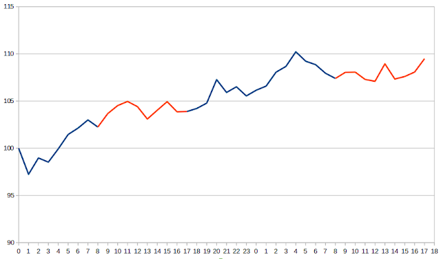
So to go from SD to ATR we'd need to multiply the SD by Y, where Y>=1. But here we can't just do some trivial adjustment. Let me explain why. Consider the following price action:

The blue line shows when the market was closed; the red line shows when it was open. The x-axis is the hour count, so the market is open between 8am and 5pm daily. The return for standard deviation purposes is the difference between the closing price on the second day (taken at 5pm) and the first day (also at 5pm):
close - close_prev = 109.48 - 103.89 = 5.59
But the true range for the second day shown will be:
max[(high-low), abs(high - close_prev), abs(low-close_prev)]
= max[(109.48 - 107.09), abs(109.48-103.89), abs(107.09-103.89)] = 5.59
In this example the two terms are equivalent. However this won't always be the case; and it's easy to construct examples where the differences aren't the same. To come up with a rule of thumb like I did before I would need to generate loads of these experiments.
[I could also do this experiment in reverse by taking the closing prices and using something like a Brownian bridge to interpolate the missing values]
However in generating the plot above I've made a key assumption which is that the volatility is the same throughout the 24 hours - and as already alluded to we can't easily make that assumption. It's more likely that the vol is lower. Here for example is another plot, but this time I've assumed that when the market is closed the vol is 1/5 of the normal value when the market isn't trading.

This is all very well, but what should the ratio of open:close volatility be? By definition it's unobservable. We could try and infer it from tracking option prices which are close to expiry, but that could well be a biased measure (people are likely to demand higher implied vol when the market is closed, since the option isn't hedgeable).
[This problem would also apply if we tried to use the brownian bridge approach]
Mapping of SD and ATR: an empirical approach
We've got as far as we can running experiments; the only thing left to do is look at some real data. Here is some pysystemtrade code. This will acquire contract level data (with HLOC prices) from quandl, and set up some futures data in mongodb, as described here. It will then measure the ATR and standard deviation, and compare the two.
I ran this over a whole bunch of futures contracts, and the magic number I got was 0.875. Basically if you have an ATR and you want to convert it to a daily standard deviation, then you multiply the ATR by 0.875. If you prefer your standard deviations annualised then multiply the ATR by 14.
It's worth thinking about how this number relates to our previous findings:
"focusing purely on the difference between square,average,square root and the mean absolute return, to go from ATR to SD you'd multiply by 1.255. In real life there are likely to be more jumps, which suggests this number would be a little bigger."
"[to account for the difference between range and true range] So to go from SD to ATR we'd need to multiply the SD by Y, where Y>=1."
In other words:
SD = ATR*0.875 [empirical]
ATR = SD*Y and SD = ATR*1.255 -> SD = ATR*1.255/Y [theory]
This suggests Y is around 1.43. I note in passing this is damn close to the square root of 2. Does this mean anything? I don't know but it's much cooler than the somewhat arbitrary 1.255.
Summary
There is no best measure of volatility. SD and ATR are just different, each with their own strengths and weaknesses. If you happen to have an ATR measure but want to use standard deviation as a risk measure then you can multiply it by 0.875. The reverse is also possible.
Incidentally I'll be using this result in my new book; to be published next year.
ATR
pysystemtrade
risk management
Statistics
Volatility