This post is all about handcrafting; a method for doing portfolio construction which human beings can do without computing power, or at least with a spreadsheet. The method aims to achieve the following goals:

carry
handcrafting
Portfolio optimization
pysystemtrade
Python
Technology
- Humans can trust it: intuitive and transparent method which produces robust weights
- Can be easily implemented by a human in a spreadsheet
- Can be back tested
- Grounded in solid theoretical foundations
- Takes account of uncertainty in data estimates
- Decent out of sample performance
- Addresses the problem of allocating capital to assets on a long only basis, or to trading strategies.
- The first post can be found here, and it motivates the need for a method like this.
- In the second post I build up the various components of the method, and discuss why they are needed.
- In the third post, I explained how you'd actually apply the method step by step, with code.
- This post will test the method with real data, addressing the question of robust weights and out of sample performance
The testing will be done using psystemtrade. If you want to follow along, get the latest version.
PS apologies for the weird formatting in this post. It's out of my hands...
PS apologies for the weird formatting in this post. It's out of my hands...
The Test Data
The test data is the 37 futures instruments in my usual data set, with the following trading rules:
- Carry
- Exponentially weighted moving average crossover (EWMAC) 2 day versus 8 day
- EWMAC 4,16
- EWMAC 8,32
- EWMAC 16,64
- EWMAC 32,128
- EWMAC 64,256
I'll be using handcrafting to calculate both the forecast and instrument weights. By the way, this isn't a very stern test of the volatility scaling, since everything is assumed to have the same volatility in a trading system. Feel free to test it with your own data.
The handcrafting code lives here (you've mostly seen this before in a previous post, just some slight changes to deal with assets that don't have enough data) with a calling function added here in my existing optimisation code (which is littered with #FIXME NEEDS REFACTORING comments, but this isn't the time or the place...).
The handcrafting code lives here (you've mostly seen this before in a previous post, just some slight changes to deal with assets that don't have enough data) with a calling function added here in my existing optimisation code (which is littered with #FIXME NEEDS REFACTORING comments, but this isn't the time or the place...).
The Competition
I will be comparing the handcrafted method to the methods already coded up in pysystemtrade, namely:
- Naive Markowitz
- Bootstrapping
- Shrinkage
- Equal weights
All the configuration options for each optimiser will be the default for pysystemtrade (you might want to read this). All optimisation will be done on an 'expanding window' out of sample basis.
from systems.provided.futures_chapter15.estimatedsystem import *
system = futures_system()
system.config.forecast_weight_estimate['method']='handcraft' # change as appropriate
system.config.instrument_weight_estimate['method']='handcraft'  # change as appropriate
del(system.config.instruments)
del(system.config.rule_variations)

system.set_logging_level("on")
Evaluating the weights
Deciding which optimisation to use isn't just about checking profitability (although we will check that in a second). We also want to see robust weights; stable, without too many zeros.
Let's focus on the forecast weights for the S&P 500 (not quite arbitrary example, this is a cheap instrument so can allocate to most of the trading rules. Looking at say instrument weights would result in a massive messy plot).
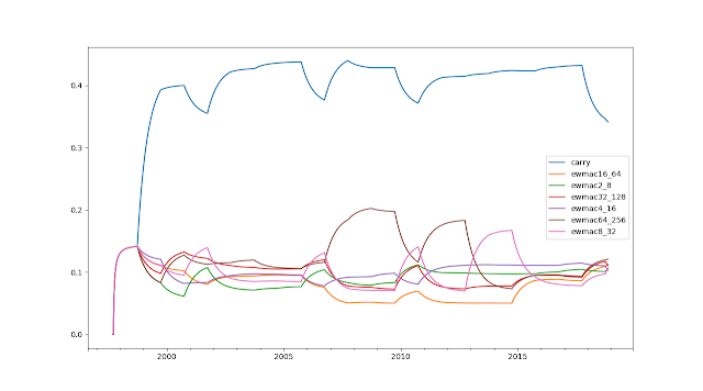
system.combForecast.get_forecast_weights("SP500") |
| Forecast weights with handcrafting |
Pretty sensible weights here, with ~35% in carry and the rest split between the other moving averages. There are some variations when the correlations shift instruments slightly between groups.
# this will give us the final Portfolio object used for optimisation (change index -1 for others)# See previous post in this series (https://qoppac.blogspot.com/2018/12/portfolio-construction-through_14.html)portfolio=system.combForecast.calculation_of_raw_estimated_forecast_weights("SP500").results[-1].diag['hc_portfolio']# eg to see the sub portfolio treeportfolio.show_subportfolio_tree()[' Contains 3 sub portfolios',
 ["[0] Contains ['ewmac16_64', 'ewmac32_128', 'ewmac64_256']"], # slow momentum
 ["[1] Contains ['ewmac2_8', 'ewmac4_16', 'ewmac8_32']"],  # fast momentum
 ["[2] Contains ['carry']"]]  # carry
Makes a lot of sense to me...
 |
| Forecast weights with naive Markowitz |
The usual car crash you’d expect from Naive Markowitz, with lots of variation, and very unrobust weights (at the end it’s basically half and half between carry and the slowest momentum). 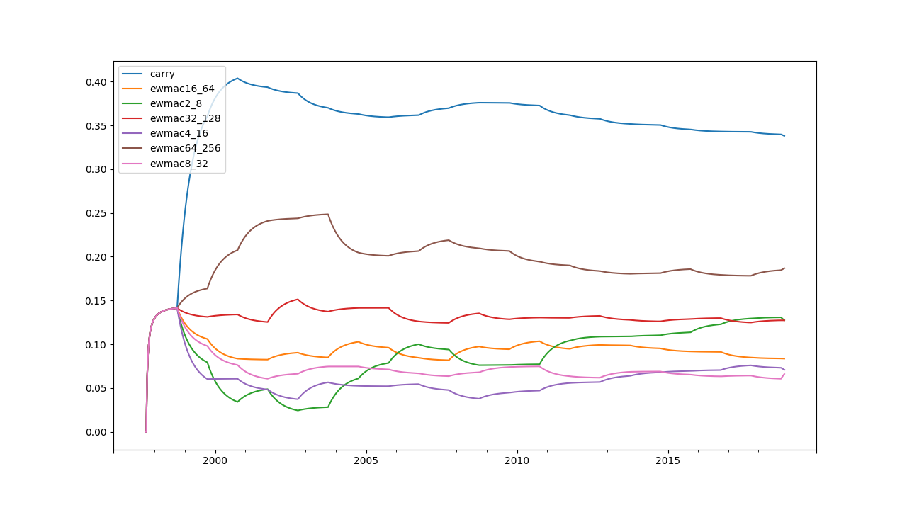 |
| Forecast weights with shrinkage |
Smooth and pretty sensible. This method downweights the faster moving averages a little more than the others; they are more expensive and also don't perform so well in equities.
 |
| Forecast weights with bootstrapping |
A lot noisier than shrinkage due to the randomness involved, but pretty sensible.
I haven't shown equal weights, as you can probably guess what those are.
Although I’m not graphing them, I thought it would be instructive to look at the final instrument weights for handcrafting:
system.portfolio.get_instrument_weights().tail(1).transpose()
AEX        0.016341
AUD        0.024343
BOBL       0.050443
BTP        0.013316
BUND       0.013448
CAC        0.014476
COPPER     0.024385
CORN       0.031373
CRUDE_W    0.029685
EDOLLAR    0.007732
EUR        0.010737
EUROSTX    0.012372
GAS_US     0.031425
GBP        0.010737
GOLD       0.012900
JPY        0.012578
KOSPI      0.031301
KR10       0.051694
KR3        0.051694
LEANHOG    0.048684
LIVECOW    0.031426
MXP        0.028957
NASDAQ     0.034130
NZD        0.024343
OAT        0.014660
PALLAD     0.013194
PLAT       0.009977
SHATZ      0.057006
SMI        0.040494
SOYBEAN    0.029706
SP500      0.033992
US10       0.005511
US2        0.031459
US20       0.022260
US5        0.007168
V2X        0.042326
VIX        0.042355
WHEAT      0.031373
Let's summarise these:
Ags 17.2%Bonds 31.8%Energy 6.1%Equities 18.3%FX 11.1%Metals 6.0%STIR 0.77%Vol 8.4%portfolio=system.portfolio.calculation_of_raw_instrument_weights().results[-1].diag['hc_portfolio']
portfolio.show_subportfolio_tree()[' Contains 3 sub portfolios', # bonds, equities, other ['[0] Contains 3 sub portfolios', # bonds ["[0][0] Contains ['BOBL', 'SHATZ']"], # german short bonds ["[0][1] Contains ['KR10', 'KR3']"], # korean bonds ['[0][2] Contains 3 sub portfolios', # other bonds ["[0][2][0] Contains ['BUND', 'OAT']"], # european 10 year bonds ex BTP ['[0][2][1] Contains 2 sub portfolios', # US medium and long bonds ["[0][2][1][0] Contains ['EDOLLAR', 'US10', 'US5']"], # us medium bonds ["[0][2][1][1] Contains ['US20']"]], # us long bond ["[0][2][2] Contains ['US2']"]]], # us short bonds ['[1] Contains 3 sub portfolios', # equities and vol ['[1][0] Contains 2 sub portfolios', # European equities ["[1][0][0] Contains ['AEX', 'CAC', 'EUROSTX']"], # EU equities ["[1][0][1] Contains ['SMI']"]], # Swiss equities ["[1][1] Contains ['NASDAQ', 'SP500']"], # US equities ["[1][2] Contains ['V2X', 'VIX']"]], # US vol ['[2] Contains 3 sub portfolios', # other ['[2][0] Contains 3 sub portfolios', # FX and metals ['[2][0][0] Contains 2 sub portfolios', # FX, mostly ["[2][0][0][0] Contains ['EUR', 'GBP']"], ["[2][0][0][1] Contains ['BTP', 'JPY']"]], ["[2][0][1] Contains ['AUD', 'NZD']"], ['[2][0][2] Contains 2 sub portfolios', # Metals ["[2][0][2][0] Contains ['GOLD', 'PALLAD', 'PLAT']"], ["[2][0][2][1] Contains ['COPPER']"]]], ['[2][1] Contains 2 sub portfolios', # letfovers ["[2][1][0] Contains ['KOSPI', 'MXP']"], ["[2][1][1] Contains ['GAS_US', 'LIVECOW']"]], ['[2][2] Contains 3 sub portfolios', # ags and crude ["[2][2][0] Contains ['CORN', 'WHEAT']"], ["[2][2][1] Contains ['CRUDE_W', 'SOYBEAN']"], ["[2][2][2] Contains ['LEANHOG']"]]]]
Some very interesting groupings there, mostly logical but a few unexpected (eg BTP, KOSPI). Also instructive to look at the smallest weights:
US10, US5, EDOLLAR, PLAT, EUR, GBP, EUROSTX (used to hedge), JPY
Those are markets I could potentially think about removing if I wanted to.
Evaluating the profits

As the figure shows the ranking of performance is as follows:
- Naive Markowitz, Sharpe Ratio (SR) 0.82
- Shrinkage, SR 0.96
- Bootstrap, SR 0.97
- Handcrafted SR 1.01
- Equal weighting SR 1.02
So naive is definitely sub optimal, but the others are pretty similar, with perhaps handcrafting and equal weights a fraction ahead of the rest. This is borne out by the T-statistics from doing pairwise comparisons between the various curves.
boot = system.accounts.portfolio() ## populate the other values in the dict below appropriatelyresults = dict(naive=oneperiodacc, hc=handcraft_acc, equal=equal_acc, shrink=shrink, boot=boot)
from syscore.accounting import account_test
types=results.keys()
for type1 in types:
for type2 in types:
if type1==type2:
continue print("%s vs %s" % (type1, type2))
print(account_test(results[type1], results[type2]))
A T-statistic of around 1.9 would hit the 5% critical value, and 2.3 is a 2% critical value):
Naive Shrink Boot HC Equal
Naive
Shrink 2.01
Boot 1.56 0.03
HC 2.31 0.81 0.58
Equal 2.33 0.97 0.93 0.19
Apart from bootstrapping, all the other methods handily beat naive with 5% significance. However the rest of the t-statistics are pretty indifferent.
Partly this is because I’ve constrained all the optimisations in similar ways so they don’t do anything too stupid; for example ignoring Sharpe Ratio when optimising over instrument weights. Changing this would mostly penalise the naive optimisation further, but probably wouldn't change things much elsewhere.
It’s always slightly depressing when equal weights beats more complicated methods, but this is partly a function of the data set. Everything is vol scaled, so there is no need to take volatility into account. The correlation structure is reasonably friendly:
- for instrument weights we have a pretty even set of instruments across different asset classes, so equal weighted and handcrafted aren’t going to be radically different,
- for forecast weights, handcrafting (and all the other methods) produce carry weights of between 30% and 40% for S&P 500, whilst equal weighting would give carry just 14%. However this difference won’t be as stark for other instruments which can only afford to trade 2 or 3 EWMAC crossovers.
Still there are many contexts in which equal weight wouldn't make sense
Incidentally the code for handcrafting runs pretty fast; only a few seconds slower than equal weights which of course is the fastest (not that pysystemtrade is especially quick... speeding it up is on my [long] to do list). Naive and bootstraps run a bit slower (as they are doing a single optimisation per time period), whilst bootstrap is slowest of all (as it’s doing 100 optimisations per time period).
Conclusion
Handcrafting produces sensible and reasonably stable weights, and it's out of sample performance is about as good as more complicated methods. The test for handcrafting was not to produce superior out of sample performance. All we needed was performance that was indistinguishable from more complex methods. I feel that it has passed this test with flying colours, albeit on just this one data set.
So if I review the original motivation for producing this method:
- - Humans can trust it; intuitive and transparent method which produces robust weights (yes, confirmed in this post)
- - Can be easily implemented by a human in a spreadsheet (yes, see post 3)
- - Can be back tested (yes, confirmed in this post)
- - Grounded in solid theoretical foundations (yes, see post 2)
- - Takes account of uncertainty (yes, see post 2)
- - Decent out of sample performance (yes, confirmed in this post)
We can see that there is a clear tick in each category. I’m pretty happy with how this test has turned out, and I will be switching the default method for optimisation in pysystemtrade to use handcrafting.